# A tibble: 6 × 2
  cuteness animal
     <dbl> <chr>
1        1 dog
2        5 cat
3        9 cat
4        3 cat
5        2 dog
6 4 horse 23 Target Encoding
23.1 Target Encoding
Target encoding (also called mean encoding, likelihood encoding, or impact encoding) is a method that maps the categorical levels to probabilities of your target variable (Micci-Barreca 2001). This method is in some ways quite similar to frequency encoding that we saw in Chapter 22. We are taking a single categorical variable, and turning it into a single numeric categorical variable.
This is a trained and supervised method since we are using the outcome of our modeling problem to guide the way this method is estimated. In the most simple formulation, target encoding is done by replacing each level of a categorical variable with the mean of the target variable within said level. The target variable will typically be the outcome, but that is not necessarily a requirement.
Consider the following example data set
If we were to calculate target encoding on animal using cuteness as the target, we would first need to calculate the mean of cuteness within each
# A tibble: 3 × 3
  animal math             mean
  <chr>  <chr>           <dbl>
1 dog    (1 + 2) / 2      1.5
2 cat    (5 + 9 + 3) / 3  5.67
3 horse  4 / 1            4
Taking these means we can now use them as an encoding
# A tibble: 6 × 2
  cuteness animal
     <dbl>  <dbl>
1        1   1.5
2        5   5.67
3        9   5.67
4        3   5.67
5        2   1.5
6        4   4
From the above example, we notice 3 things. Firstly, once the calculations have been done, applying the encoding to new data is a fairly easy procedure as it amounts to a left join. Secondly, some classes have different numbers of observations associated with them. The "horse" class only has 1 observation in this data set, how confident are we that the mean calculated from this value is as valid as the mean that was calculated over the 3 values for the "cat" class? Lastly, how will this method handle unseen levels?
Let us think about the unseen levels first. If we have no information about a given class. This could happen in at least two different ways. Because the level is truly unseen because the company was just started and wasn’t known in the training data set. Or because the known level wasn’t observed, e.i. no Sundays in the training data set. Regardless of the reason, we will want to give these levels a baseline number. For this, we can use the mean value of the target, across all of the training data set. So for our toy example, we have a mean cuteness of 4, which we will assign to any new animal.
This value is by no means a good value, but it is an educated guess that can be calculated with ease. This also means that regardless of the distribution of the target, these values can be calculated.
The way we handle unseen levels gives us a clue as to how we can deal with low-frequency counts. Knowing that the global mean of the target is our baseline when we have no information. We can combine the level mean with the global mean, in accordance with how many observations we observe. If we have a lot of observations at a level, we will let the global mean have little influence, and if there are fewer observations we will let the global mean have a higher influence.
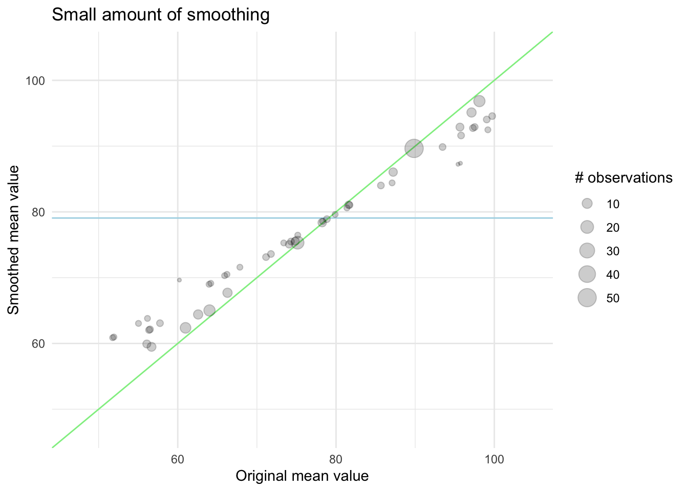
We can visualize this effect in the following charts. First, we have an example of what happens with a smaller amount of smoothing. The points are mostly along the diagonal. Remember that if we didn’t do this, all the points would be along the diagonal regardless of their size.

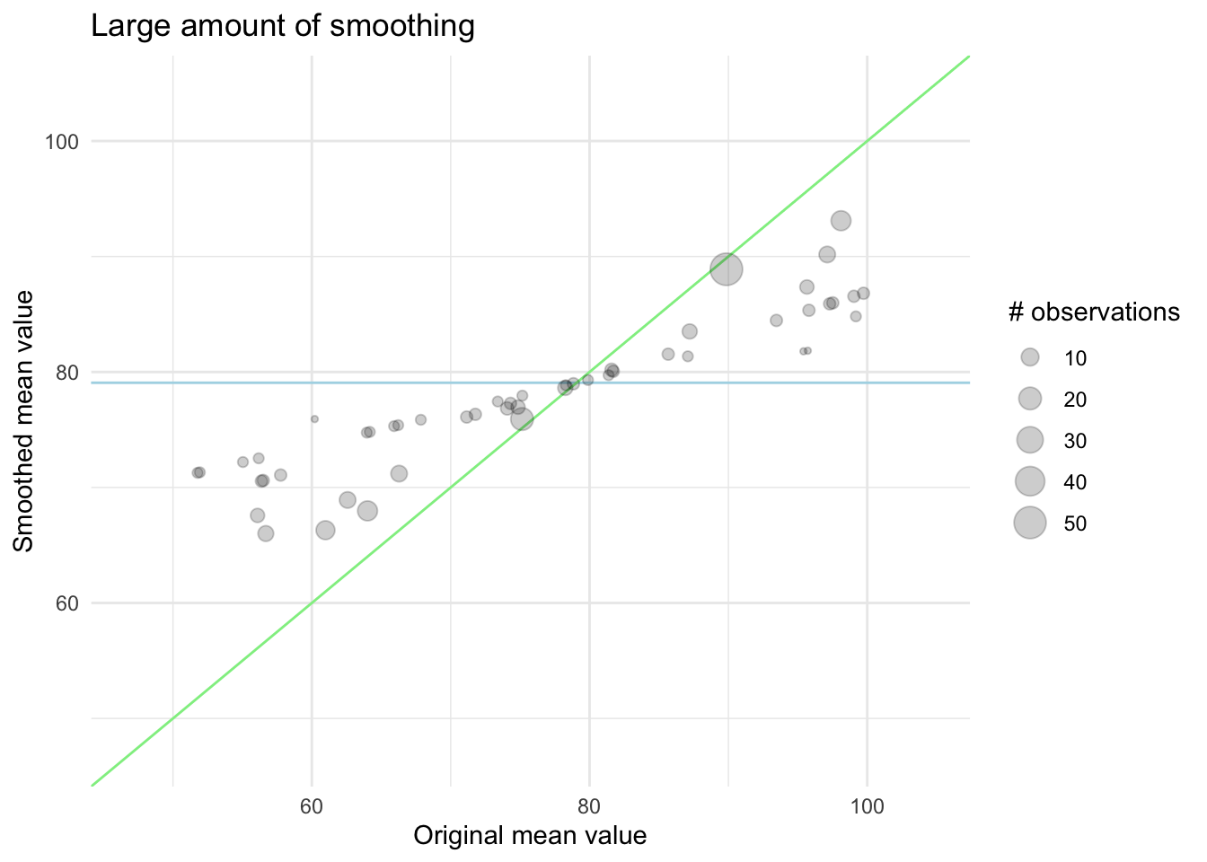
In this next chart, we see the effect of a higher amount of smoothing, now the levels with fewer observations are pulled quite a bit closer to the global mean.

The exact way this is done will vary from method to method, and the strength of this smoothing can and should properly be tuned as there isn’t an empirical best way to choose it.
This smoothing isn’t required but it is often beneficial to include if you are dealing with low count levels. It is also recommended because if omitted, it would lead to overfitting since we are essentially using the outcome to guide the predictors.
We have so far talked about target encoding, from the perspective of a regression task. But target encoding is not limited to numeric outcomes, but can be used in classification settings as well. In the classification setting, where we have a categorical outcome, instead of calculating the mean of the target variable, we need to figure something else out. It could be calculating the probability of the first level, or we could try to go more linear by converting them to log odds. Now everything works as before.
find good example
A type of data that is sometimes seen is hierarchical categorical variables. Typical examples are city-state and region-subregion. With hierarchical categorical variables you often end up with many levels, and target encoding can be used on such data, and can even use the hierarchical structure.
The encoding is calculated like normal, but the smoothing is done on a lower level than at the top. So instead of adjusting by the global mean, you smooth by the level below it.
23.2 Pros and Cons
23.2.1 Pros
- Can deal with categorical variables with many levels
- Can deal with unseen levels in a sensible way
23.2.2 Cons
- Can be prone to overfitting
23.3 R Examples
The embed package comes with a couple of functions to do target encoding. step_lencode_glm(), step_lencode_bayes() and step_lencode_mixed(). These functions are named such because they likelihood encode variables, and because the encodings can be calculated using no intercept models.
step_lencode_glm() implements the no-smoothing method, so we will look at that one first using the ames data set.
find a better data set
library(recipes)
library(embed)

data(ames, package = "modeldata")

rec_target <- recipe(Sale_Price ~ Neighborhood, data = ames) |>
  step_lencode_glm(Neighborhood, outcome = vars(Sale_Price)) |>
  prep()

rec_target |>
  bake(new_data = NULL)
# A tibble: 2,930 × 2
Neighborhood Sale_Price
<dbl> <int>
1 145097. 215000
2 145097. 105000
3 145097. 172000
4 145097. 244000
5 190647. 189900
6 190647. 195500
7 324229. 213500
8 324229. 191500
9 324229. 236500
10 190647. 189000
# ℹ 2,920 more rowsAnd we see that it works as intended, we can pull out the exact levels using the tidy() method
rec_target |>
  tidy(1)
# A tibble: 29 × 4
level value terms id
<chr> <dbl> <chr> <chr>
1 North_Ames 145097. Neighborhood lencode_glm_Bp5vK
2 College_Creek 201803. Neighborhood lencode_glm_Bp5vK
3 Old_Town 123992. Neighborhood lencode_glm_Bp5vK
4 Edwards 130843. Neighborhood lencode_glm_Bp5vK
5 Somerset 229707. Neighborhood lencode_glm_Bp5vK
6 Northridge_Heights 322018. Neighborhood lencode_glm_Bp5vK
7 Gilbert 190647. Neighborhood lencode_glm_Bp5vK
8 Sawyer 136751. Neighborhood lencode_glm_Bp5vK
9 Northwest_Ames 188407. Neighborhood lencode_glm_Bp5vK
10 Sawyer_West 184070. Neighborhood lencode_glm_Bp5vK
# ℹ 19 more rowsto apply smoothing we can use the step_lencode_mixed() step in the same way
rec_target_smooth <- recipe(Sale_Price ~ Neighborhood, data = ames) |>
  step_lencode_mixed(Neighborhood, outcome = vars(Sale_Price)) |>
  prep()

rec_target_smooth |>
  bake(new_data = NULL)
# A tibble: 2,930 × 2
Neighborhood Sale_Price
<dbl> <int>
1 145156. 215000
2 145156. 105000
3 145156. 172000
4 145156. 244000
5 190633. 189900
6 190633. 195500
7 322591. 213500
8 322591. 191500
9 322591. 236500
10 190633. 189000
# ℹ 2,920 more rowsWe see that these values are slightly different than the values we had earlier
rec_target_smooth |>
  tidy(1)
# A tibble: 29 × 4
level value terms id
<chr> <dbl> <chr> <chr>
1 North_Ames 145156. Neighborhood lencode_mixed_RUieL
2 College_Creek 201769. Neighborhood lencode_mixed_RUieL
3 Old_Town 124154. Neighborhood lencode_mixed_RUieL
4 Edwards 131021. Neighborhood lencode_mixed_RUieL
5 Somerset 229563. Neighborhood lencode_mixed_RUieL
6 Northridge_Heights 321519. Neighborhood lencode_mixed_RUieL
7 Gilbert 190633. Neighborhood lencode_mixed_RUieL
8 Sawyer 136956. Neighborhood lencode_mixed_RUieL
9 Northwest_Ames 188401. Neighborhood lencode_mixed_RUieL
10 Sawyer_West 184085. Neighborhood lencode_mixed_RUieL
# ℹ 19 more rows23.4 Python Examples
We are using the ames data set for examples. {sklearn} provided the TargetEncoder() method we can use. For this to work, we need to remember to specify an outcome when we fit().
from feazdata import ames
from sklearn.compose import ColumnTransformer
from sklearn.preprocessing import TargetEncoder

ct = ColumnTransformer(
    [('target', TargetEncoder(target_type="continuous"), ['Neighborhood'])],
    remainder="passthrough")

ct.fit(ames, y=ames[["Sale_Price"]].values.flatten())
ColumnTransformer(remainder='passthrough',
transformers=[('target',
TargetEncoder(target_type='continuous'),
['Neighborhood'])])In a Jupyter environment, please rerun this cell to show the HTML representation or trust the notebook. On GitHub, the HTML representation is unable to render, please try loading this page with nbviewer.org.
ColumnTransformer(remainder='passthrough',
                  transformers=[('target',
                                 TargetEncoder(target_type='continuous'),
['Neighborhood'])])['Neighborhood']
TargetEncoder(target_type='continuous')
['MS_SubClass', 'MS_Zoning', 'Lot_Frontage', 'Lot_Area', 'Street', 'Alley', 'Lot_Shape', 'Land_Contour', 'Utilities', 'Lot_Config', 'Land_Slope', 'Condition_1', 'Condition_2', 'Bldg_Type', 'House_Style', 'Overall_Cond', 'Year_Built', 'Year_Remod_Add', 'Roof_Style', 'Roof_Matl', 'Exterior_1st', 'Exterior_2nd', 'Mas_Vnr_Type', 'Mas_Vnr_Area', 'Exter_Cond', 'Foundation', 'Bsmt_Cond', 'Bsmt_Exposure', 'BsmtFin_Type_1', 'BsmtFin_SF_1', 'BsmtFin_Type_2', 'BsmtFin_SF_2', 'Bsmt_Unf_SF', 'Total_Bsmt_SF', 'Heating', 'Heating_QC', 'Central_Air', 'Electrical', 'First_Flr_SF', 'Second_Flr_SF', 'Gr_Liv_Area', 'Bsmt_Full_Bath', 'Bsmt_Half_Bath', 'Full_Bath', 'Half_Bath', 'Bedroom_AbvGr', 'Kitchen_AbvGr', 'TotRms_AbvGrd', 'Functional', 'Fireplaces', 'Garage_Type', 'Garage_Finish', 'Garage_Cars', 'Garage_Area', 'Garage_Cond', 'Paved_Drive', 'Wood_Deck_SF', 'Open_Porch_SF', 'Enclosed_Porch', 'Three_season_porch', 'Screen_Porch', 'Pool_Area', 'Pool_QC', 'Fence', 'Misc_Feature', 'Misc_Val', 'Mo_Sold', 'Year_Sold', 'Sale_Type', 'Sale_Condition', 'Sale_Price', 'Longitude', 'Latitude']
passthrough
ct.transform(ames).filter(regex="target.*") target__Neighborhood
0 145110.156
1 145110.156
2 145110.156
3 145110.156
4 190636.427
... ...
2925 162269.818
2926 162269.818
2927 162269.818
2928 162269.818
2929 162269.818
[2930 rows x 1 columns]